2.3 Feature Analysis
2.3.1 Feature Distribution
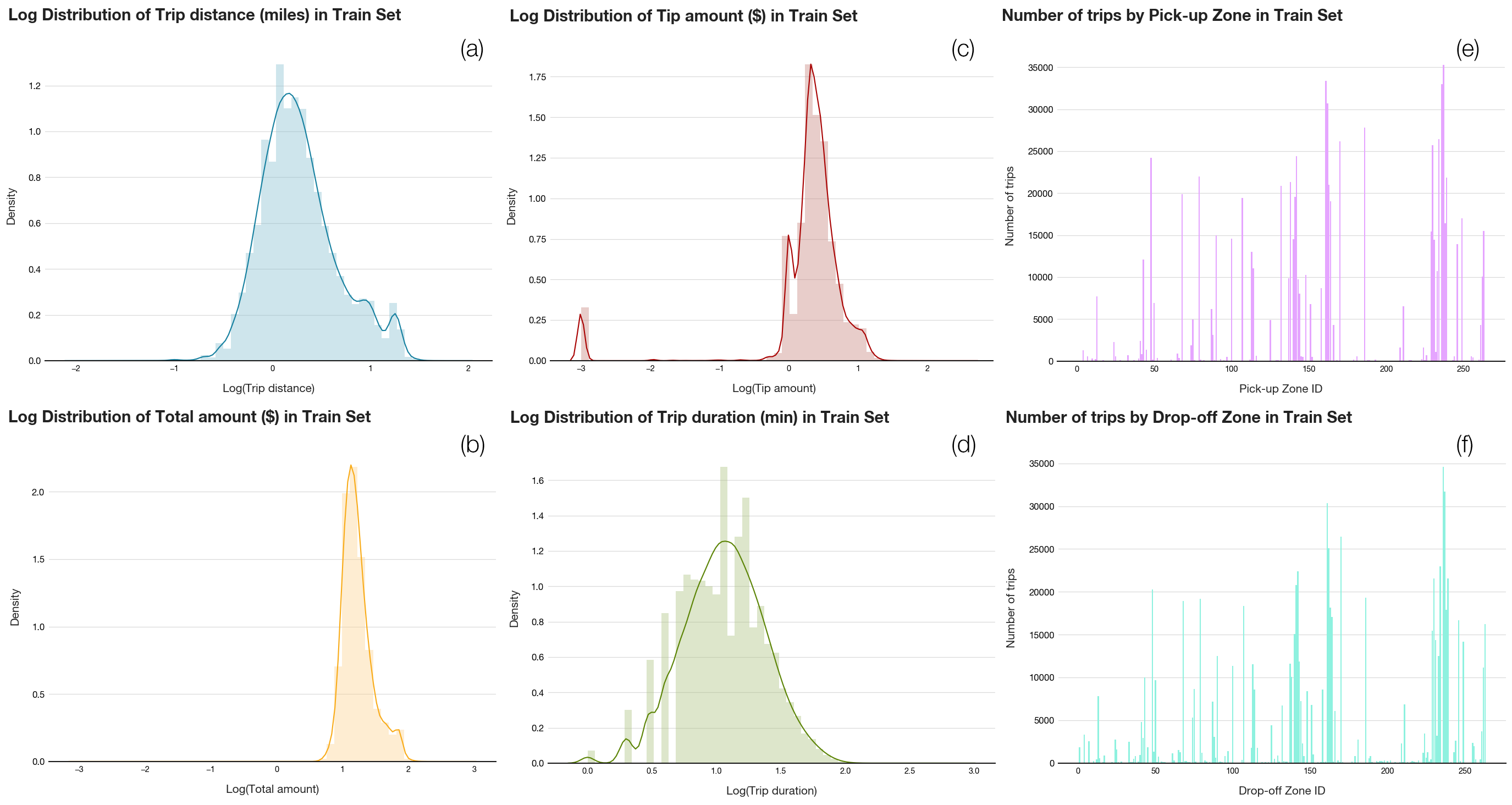
Figure 1. Feature log distributions
Figure 1 shows the distributions of the main six features to be included in the modelling phase. The distributions, which come from the training set, demonstrate similar trends in the distributions visualized in phase 1 of the project, specifically:
- Trip distance and Total amount display bimodality (a and b), with the lower mode corresponding to the airport trips. These trips typically cost around $52, or equivalently 1.72 in log scale.
- More than a quarter of trips have a log Tip amount of -3 (c), which means no tips were included in the original transactions.
- The missing gaps in the duration distribution (d) are due to the nearest integer rounding when this feature was engineered in phase 1. As such, the shape of the distribution is not abnormal. Note that the bimodality due to airport trips is not strongly exhibited for this feature.
- Even without a choropleth map, the demand in the three hotspot areas is transparent from the raw count of trips per zone (e and f). Areas with high pick-up demand usually imply high drop-off demand correspondingly.
It is also worth noticing that none of the transformed distribution for the numerical features (Distance, tip amount, total amount, duration) are approximately normal. Two tests for normality, D’Agostino’s K-squared test 18 and Shapiro–Wilk test 19, are performed on each feature in both the training and the testing sets using the scipy Python package and detected no normality with extremely high statistical significance. This insight helps with the choice of models in the modelling section below.
2.3.2 Pairwise Correlation
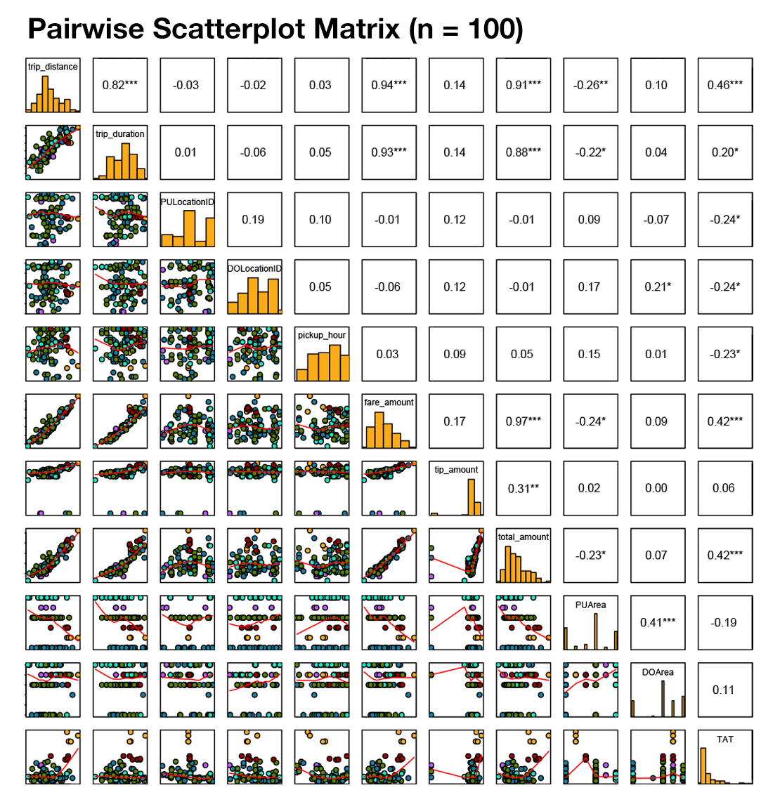
Figure 2. Pairwise scatterplot matrix colored by pickup areas
A sample of 100 points from the training set was plotted on a pairwise scatter-plot matrix, colored by pickup areas (Figure 2). As expected, all numerical features have statistically significant multicollinearity with each other, barring the instances with no tip. As our target variable is Total amount, it means that only one of Distance, Fare Amount, Tip Amount, and Duration should be included in the model so that coefficient estimates are not affected by scaling (see Feature Selection below). Furthermore, Total amount seems to be randomly distributed across different zones and pick-up hours, suggesting that these features may not be suitable predictors for the model. TAT is moderately linear to Total amount and shows clear interaction with pick-up areas from the coloring. Specifically, TAT and Total amount for airport areas are noticeably higher that the other areas.
2.3.3 Comparison of Spatial Resolution
While visualizing the data on a zone-based resolution is effective in phase 1, the high cardinality of 250 different zones presents a challenge in model training. As such, a broader segmentation of location is proposed by grouping the zones into 6 areas: Downtown, Midtown, Uptown, LGA, JFK, Others. Although the initial plan was to compare the effectiveness of these two grouping strategies, the curse of dimensionality 20 introduced by the number of zones bore an immense time complexity cost on training even the minimal dataset. Thus, this analysis is done pre-emptively to ensure that area-based grouping will not lose much information compared to zone-based grouping. As the analysis lends itself to the idea of information gain from information theory, the normalized mutual information (NMI) will be used as the metric for comparison 21.
The Total amount is cut to 100000 bins, before being used to calculate the NMI with each of PULocationID, PUArea, DOLocationID, DOArea. While area-based grouping indeed results in information loss (see the NMI result table above), the trade-off between the loss and the reduction in training time as well as model simplicity is well-worth the use of area-based grouping over zone-based grouping strategy.
2.3.4 Categorical – Numerical Feature Interactions
Figure 2 implies that Total amount is somewhat affected by areas. Specifically, the median values for the airports are higher than the remaining areas, suggesting a higher slope for these two areas. However, they also recorded the largest number of outliers despite having a relatively lower IQR spread, which means that the mean error from predictions will be expectedly higher than the other areas. Such interaction is statistically supported using the Kruskal-Wallis test by ranks, a non-parametric equivalence of the one-way ANOVA 22, on the 100-instance subsample \((\chi^2(5)=22.413, p=.0004)\).
Furthermore, the boxplot also raises a concern about malicious data points that may distort the model fit. A subjective threshold of 2.3 (equivalently a trip total amount of $200) was used as a cut-off to rule out any potential outliers to the training set. An investigation into these outliers indicates that, while some are genuinely due to long trip distance and duration, there are some highly generous customers whose tips are nearly tenfold the fare amount. As these trips do not honour the typical relationship with Total amount, we further remove trips with outlier tip-to-total ratios from the training set. As a result, 799925 instances remain in the training set.
2.3.5 Feature Selection for Explanatory Models
From the feature analysis, we rule out PULocationID, DOLocationID and pickup_hour from the predictors pool. Amongst the numerical features, Trip Duration seems to be the most suitable one, as a driver can usually estimate how long the trip will take prior to picking up the passengers. Trip Distance can be estimated with the interaction between PUArea and DOArea, while Fare Amount and Tip Amount are only known after the trip has taken place, and thus do not make sense to be included in a regression model.
The set of predictors X for the explanatory modelling phase is finalized as: Duration, PUArea, DOArea, TAT.
d’Agostino, R. B. (1971). An omnibus test of normality for moderate and large size samples. Biometrika, 58(2), 341-348.↩︎
Razali, N. M., & Wah, Y. B. (2011). Power comparisons of shapiro-wilk, kolmogorov-smirnov, lilliefors and anderson-darling tests. Journal of statistical modeling and analytics, 2(1), 21-33.↩︎
Verleysen, M., & François, D. (2005, June). The curse of dimensionality in data mining and time series prediction. In International work-conference on artificial neural networks (pp. 758-770). Springer, Berlin, Heidelberg.↩︎
Strehl, A., & Ghosh, J. (2002). Cluster ensembles—a knowledge reuse framework for combining multiple partitions. Journal of machine learning research, 3(Dec), 583-617.↩︎
Kruskal, W. H., & Wallis, W. A. (1952). Use of ranks in one-criterion variance analysis. Journal of the American statistical Association, 47(260), 583-621.↩︎